DDCASPT2

In this tutorial, the potential energy curve of the symmetric angle bend of ozone is shown using data-driven complete active space second-order perturbation theory (DDCASPT2).

Link to the code repository: DDQC Demo

Required python3 modules:

matplotlib
numpy
pandas
seaborn
os
pickle
sklearn
mpl_toolkits

If you are missing any of these packages, we would recommend using the following lines in your juypter notebook:

import sys
!{sys.executable} -m pip install missing_package_name

Import packages

# Visualization packages
import matplotlib.pyplot as plt
import seaborn as sns; sns.set(style="ticks", color_codes=True)
from mpl_toolkits.axes_grid.inset_locator import (inset_axes, InsetPosition,mark_inset)

# Misc. packages
import numpy as np
import pandas as pd
import os
import pickle5 as pickle



# Regressor
from sklearn.ensemble import RandomForestRegressor
# Preprocessing
from sklearn.preprocessing import MinMaxScaler
from sklearn.model_selection import train_test_split
# Metrics
from sklearn.metrics import mean_absolute_error
from sklearn.metrics import mean_squared_error
from sklearn.metrics import r2_score

Files required to run gen_pair.ipynb:

The angles (106-180 degrees): keys.pickle
The regression targets Y (pair energies): targets.pickle
The feature set, X: feats.pickle
True CASSCF energies: casscf.csv
True CASPT2 energies: caspt2.csv
The true correlation energies (E2): E2.csv

with open('feats.pickle', 'rb') as handle:
    X = pickle.load(handle)

with open('targets.pickle', 'rb') as handle:
    Y = pickle.load(handle)

with open('keys.pickle', 'rb') as handle:
    keys = pickle.load(handle)

angles=np.arange(106,181,1)
l=keys
l=[i for i in l if float(i)>=110.0 and float(i)<=170.0]
print(f'Number of data points in potential energy curve: {len(l)}')

# Split the data 70% train/30% test
train_ind,test_ind=train_test_split(l, test_size=0.3, random_state=0)
num_train=[int(i) for i in np.linspace(10,len(train_ind),19)]


X_train=X.loc[train_ind].to_numpy()
X_test=X.loc[test_ind].to_numpy()

y_train=Y[train_ind].T.stack().to_numpy()
y_test=Y[test_ind].T.stack().to_numpy()

caspt2=pd.read_csv('caspt2.csv',index_col='Label').drop(columns='Unnamed: 0')
casscf=pd.read_csv('casscf.csv',index_col='Label').drop(columns='Unnamed: 0').loc[map(float,test_ind)].rename(columns={'SCF':0})
E1Dict=pd.read_csv("E2.csv").rename(columns={'Unnamed: 0':'Label'}).set_index('Label')

First Evaluation Metric

Features are scaled and then a random forest regressor is trained to predict pair energies. 70% of the data for training and 30% for testing.

scaler = MinMaxScaler().fit(X_train)
X_train_scaled = scaler.transform(X_train)
X_test_scaled = scaler.transform(X_test)
regr = RandomForestRegressor(max_depth=1000,max_features='sqrt',bootstrap=True,oob_score=True,n_estimators=700,random_state =69,n_jobs=-1).fit(X_train_scaled, y_train)
y_train_pred=regr.predict(X_train_scaled)
y_test_pred=regr.predict(X_test_scaled)

plt.figure(figsize=(10,5))
plt.subplot(1, 2, 1)
fill=np.linspace(min(y_test)-1e-2,max(y_test)+1e-2,20)
plt.plot(fill,fill,color='black',alpha=0.75)
plt.fill_between(fill,fill-0.0016,fill+0.0016,color='gray', alpha=0.3)
plt.fill_between(fill,fill-0.003665,fill+0.003665,color='darkgray', alpha=0.3)

plt.scatter(y_train,y_train_pred,alpha=1,marker='.')
plt.xticks(np.round(np.linspace(min(y_train), max(y_train), 4),4),rotation=0)
plt.text(min(y_train), max(y_train)-5e-3, f'R$^{2}$: {r2_score(y_train,y_train_pred):0.3f}',fontsize=12,bbox=dict(facecolor='white', alpha=1.0))
plt.xlim(min(y_train)-1e-3, max(y_train)+1e-3)
plt.ylim(min(y_train)-1e-3, max(y_train)+1e-3)
plt.xlabel('True pair-energies (E$_{h}$)',fontsize=12)
plt.ylabel('Predicted pair-energies (E$_{h}$)',fontsize=12)
plt.title('O$_{3}$ (4,3) VDZP 1D Train Set',fontsize=12)
plt.subplot(1, 2, 2)
fill=np.linspace(min(y_test)-1e-2,max(y_test)+1e-2,20)
plt.plot(fill,fill,color='black',alpha=0.75)
plt.fill_between(fill,fill-0.0016,fill+0.0016,color='gray', alpha=0.3)
plt.fill_between(fill,fill-0.003665,fill+0.003665,color='darkgray', alpha=0.3)
plt.scatter(y_test,y_test_pred,alpha=1,marker='.',color='orange')
plt.xticks(np.round(np.linspace(min(y_test), max(y_test), 4),4),rotation=0)
plt.text(min(y_test), max(y_test)-5e-3, f'R$^{2}$: {r2_score(y_test,y_test_pred):0.3f}',fontsize=12,bbox=dict(facecolor='white', alpha=1.0))
plt.xlim(min(y_test)-1e-3, max(y_test)+1e-3)
plt.ylim(min(y_test)-1e-3, max(y_test)+1e-3)
plt.xlabel('True pair-energies (E$_{h}$)',fontsize=12)
plt.ylabel('Predicted pair-energies (E$_{h}$)',fontsize=12)
plt.title('O$_{3}$ (4,3) VDZP 1D Test Set',fontsize=12)

plt.tight_layout()
plt.show()

Test set on the potential energy curve

The pair energies (\(\varepsilon_{pq}\)) predicted from the test set can then be summed into correlation energies (\(E_{2}\)):

\[E_{2}=\sum_{pq} \varepsilon_{pq}\]

pred_train_E2=np.sum(y_train_pred.reshape(len(train_ind),-1),axis=1)
train_E2=np.sum(y_train.reshape(len(train_ind),-1),axis=1)
pred_test_E2=np.sum(y_test_pred.reshape(len(test_ind),-1),axis=1)
test_E2=np.sum(y_test.reshape(len(test_ind),-1),axis=1)

df_PredE2=pd.DataFrame(pred_test_E2,index=map(float,test_ind))

plt.plot(caspt2-caspt2.max().values,label='CASPT2')
plt.scatter(list(map(float,test_ind)),casscf.add(df_PredE2,fill_value=0)-caspt2.max().values,label='DDCASPT2',color='red')
plt.legend()
plt.title(r'O$_{3}$ Potential Energy Curve',fontsize=14)
plt.ylabel('Energy (E$_{h}$)',fontsize=14)
plt.xlabel('Bond Degrees ($^{\circ}$)',fontsize=14)
plt.tight_layout()
plt.show()

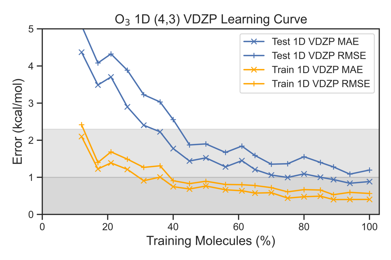
Second Evaluation Metric

Learning curves are used to evaluate the effectiveness of our model with respect to the total correlation energies. The amount of test data is held the same as training set is systematically increased.

# Create the dataset
rng = np.random.default_rng(42)
# factor_dict=pd.read_excel('factor_dict.xlsx')
R2=[]
MAE=[]
RMSE=[]
kcalMAE=[]
kcalRMSE=[]
Train_R2=[]
Train_MAE=[]
Train_RMSE=[]
Train_kcalMAE=[]
Train_kcalRMSE=[]
Num_Test=[]
Num_Train=[]
for k in num_train:
    TestE2_list=[]
    PredE2_list=[]
    Train_E2_list=[]
    Train_PredE2_list=[]
    testsubs_list=[]
    trainsubs_list=[]


    print(f'Number of Train {k}')
#         trainsubs=random.sample(train_ind, k)
    trainsubs=train_ind[0:k]
    testsubs=test_ind
    Num_Test.append(len(testsubs))
    Num_Train.append(k)
    print(f'Number of test {len(testsubs)}')
#         for typ in ['A','B','C','D','E','F','G','H']:
    
    y=Y
    X_test_stacked=X.loc[testsubs].to_numpy()
    X_train_stacked=X.loc[trainsubs].to_numpy()
    y_test_stacked=y[testsubs].T.stack().to_numpy()
    y_train_stacked=y[trainsubs].T.stack().to_numpy()


    test_labels=testsubs
    train_labels=trainsubs
    scaler = MinMaxScaler().fit(X_train_stacked)
    X_train_scaled = scaler.transform(X_train_stacked)
    X_test_scaled = scaler.transform(X_test_stacked)
    print(X_train_scaled.shape)
#     reg8=KNeighborsRegressor(n_neighbors=int(np.log(len(y[trainsubs[0]]))),leaf_size=1,n_jobs=-1,p=1).fit(X_train_scaled,y_train_stacked)    
    reg8=regr.fit(X_train_scaled,y_train_stacked)
#     reg8=RandomForestRegressor(max_features='sqrt',bootstrap=True,oob_score=True,n_estimators=700,random_state =69,n_jobs=-1).fit(X_train_scaled, y_train_stacked)
    
    print(reg8.get_params)
    y_test_trimpred=reg8.predict(X_test_scaled)
    y_train_trimpred=reg8.predict(X_train_scaled)


    print('pair energies (e\u2082) test R\u00b2: %.4f' %r2_score(y_test_stacked,y_test_trimpred))
    print('pair energies (e\u2082) train R\u00b2: %.4f' %r2_score(y_train_stacked,y_train_trimpred))  
    PredE2=np.sum(y_test_trimpred.reshape(len(testsubs),-1),axis=1)
    TestE2=np.sum(y_test_stacked.reshape(len(testsubs),-1),axis=1)
    Train_PredE2=np.sum(y_train_trimpred.reshape(len(trainsubs),-1),axis=1)
    Train_E2=np.sum(y_train_stacked.reshape(len(trainsubs),-1),axis=1)
    TestE2_list.append(TestE2)
    PredE2_list.append(PredE2)
    Train_E2_list.append(Train_E2)
    Train_PredE2_list.append(Train_PredE2)
    testsubs_list.append(testsubs)
    trainsubs_list.append(trainsubs)
    

    R2.append(r2_score(TestE2,PredE2))
    MAE.append(mean_absolute_error(TestE2,PredE2))
    RMSE.append(np.sqrt(mean_squared_error(TestE2,PredE2)))
    kcalMAE.append(627.5*mean_absolute_error(TestE2,PredE2))
    kcalRMSE.append(627.5*np.sqrt(mean_squared_error(TestE2,PredE2)))

    Train_R2.append(r2_score(Train_E2,Train_PredE2))
    Train_MAE.append(mean_absolute_error(Train_E2,Train_PredE2))
    Train_RMSE.append(np.sqrt(mean_squared_error(Train_E2,Train_PredE2)))
    Train_kcalMAE.append(627.5*mean_absolute_error(Train_E2,Train_PredE2))
    Train_kcalRMSE.append(627.5*np.sqrt(mean_squared_error(Train_E2,Train_PredE2)))

    print('Test E\u2082 MAE: %.4E' % mean_absolute_error(TestE2,PredE2), 'E\u2095')
    print('Test E\u2082 RMSE: %.4E' % np.sqrt(mean_squared_error(TestE2,PredE2)), 'E\u2095','\n')
    print('Test E\u2082 MAE: %.4E' % ((mean_absolute_error(TestE2,PredE2))*627.5), 'kcal/mol')
    print('Test E\u2082 RMSE: %.4E' % (np.sqrt(mean_squared_error(TestE2,PredE2))*627.5), 'kcal/mol','\n')

    print('Train E\u2082 MAE: %.4E' % mean_absolute_error(Train_E2,Train_PredE2), 'E\u2095')
    print('Train E\u2082 RMSE: %.4E' % np.sqrt(mean_squared_error(Train_E2,Train_PredE2)), 'E\u2095','\n')
    print('Train E\u2082 MAE: %.4E' % ((mean_absolute_error(Train_E2,Train_PredE2))*627.5), 'kcal/mol')
    print('Train E\u2082 RMSE: %.4E' % (np.sqrt(mean_squared_error(Train_E2,Train_PredE2))*627.5), 'kcal/mol','\n')
    
#     pd.DataFrame({'TestE2':TestE2,'testsubs':testsubs,'PredE2':PredE2}).to_excel(f'big_scaled_super_4_3_VDZP_Test_Energies.xlsx')
#     pd.DataFrame({'Num_Test':Num_Test,'Num_Train':Num_Train,'Test_R2':R2,'Test_MAE (kcal/mol)':kcalMAE,'Test_RMSE (kcal/mol)':kcalRMSE,'Test_MAE (Eh)':MAE,'Test_RMSE (Eh)':RMSE,'Train_R2':Train_R2,'Train_MAE':Train_MAE,'Train_RMSE':Train_RMSE,'Train_kcalMAE':Train_kcalMAE,'Train_kcalRMSE':Train_kcalRMSE}).sort_values('Num_Train').to_excel(f'big_scaled_super_4_3_VDZP_Learning_Curve_1D.xlsx')

df = pd.DataFrame({'Num_Test':Num_Test,'Num_Train':Num_Train,'Test_R2':R2,'Test_MAE (kcal/mol)':kcalMAE,'Test_RMSE (kcal/mol)':kcalRMSE,'Test_MAE (Eh)':MAE,'Test_RMSE (Eh)':RMSE,'Train_R2':Train_R2,'Train_MAE':Train_MAE,'Train_RMSE':Train_RMSE,'Train_kcalMAE':Train_kcalMAE,'Train_kcalRMSE':Train_kcalRMSE}).sort_values('Num_Train')
test=pd.DataFrame({'TestE2':TestE2,'testsubs':testsubs,'PredE2':PredE2}).set_index('testsubs')

      
# df = pd.read_excel(f'big_scaled_super_4_3_VDZP_Learning_Curve_1D.xlsx',engine='openpyxl')
# test=pd.read_excel('big_scaled_super_4_3_VDZP_Test_Energies.xlsx',engine='openpyxl').set_index('testsubs').drop(columns='Unnamed: 0')
VDZP_perc_train=[float(f'{i*100:0.0f}') for i in list(df['Num_Train']/df['Num_Train'].iloc[-1])]
VDZP_test_R2=df['Test_R2']
VDZP_Train_R2=df['Train_R2']
VDZP_Test_MAE=df['Test_MAE (kcal/mol)']
VDZP_Test_RMSE=df['Test_RMSE (kcal/mol)']
VDZP_train_MAE=df['Train_kcalMAE']
VDZP_train_RMSE=df['Train_kcalRMSE']

plt.plot(VDZP_perc_train,VDZP_Test_MAE,color='b',label=f'Test 1D VDZP MAE',marker='x')
plt.plot(VDZP_perc_train,VDZP_Test_RMSE,color='b',label=f'Test 1D VDZP RMSE',marker='+')
plt.plot(VDZP_perc_train,VDZP_train_MAE,color='orange',label=f'Train 1D VDZP MAE',marker='x')
plt.plot(VDZP_perc_train,VDZP_train_RMSE,color='orange',label=f'Train 1D VDZP RMSE',marker='+')


plt.title(r'O$_{3}$ 1D (4,3) VDZP Learning Curve',fontsize=14)
plt.xlabel(r'Training Molecules (%)',fontsize=14)
plt.ylabel(r'Error (kcal/mol)',fontsize=14)
plt.xlim(0,103)
plt.ylim(0,5)
plt.fill_between(np.arange(-1,105),0, 1,color='gray', alpha=0.3)
plt.fill_between(np.arange(-1,105),1, 2.3,color='darkgray', alpha=0.3)

plt.legend(loc=1)
plt.tight_layout()
plt.show()